Portfolio Optimization Based on Sharpe Ratio and Genetic Algorithm
This post shows the application of the theory of genetic algorithms to an optimization problem of a portfolio of shares. Both the optimization problems and the theory of genetic algorithms are exposed briefly and are useful to solve specific problems, to find the best assignment when it is necessary to invest. The exposition of this interesting topic is helped by software that allows seeing the step-by-step optimization process by using genetic algorithms.
For the present post, we use the portfolio selection model of Markowitz (1952), using the performance measurement for mutual fund portfolios proposed by Sharpe (1964), a measure that was originally called reward-to-variability ratio and became popular as Sharpe’s index, measure, or ratio. The following are the basic elements of the Markowitz portfolio selection model and the Sharpe ratio as a measure of performance and optimization of the return/risk ratio.
Table of contents:
Introduction
Stock selection is a critically important issue when it comes to investing in the stock market, and the first problem that investors encounter. When investors select stocks, they consider the risk and the return of the stock. However, a single stock with a high return usually entails high risk, while a single stock with low risk entails low return. Investors naturally want to invest in stocks with low risk and high return. The fluctuation of stock price can represent the risk of this stock. As the proverb says, “Do not put all your eggs in one basket.” In order to stabilize the fluctuation of stocks, we aggregate different stocks in a portfolio because a good combination of stocks is able to reduce the holistic risk and increase the return. Therefore, this post provides a portfolio that simultaneously considers risk and return to investors.
Modern Portfolio Theory
The concept of diversification was formalized with the Modern Theory of Finance. This is how Markowitz (1952) presented a portfolio selection model that incorporated the principles of diversification, identifying a set of efficient portfolios, or the efficient frontier of risky assets. The main idea of this set of risky portfolios is that, for any level of risk, only the portfolio with the highest expected return is of interest. Alternatively, the frontier is the set of portfolios that minimizes the variance for any expected return goal.
The application of this model corresponds, in the first instance, to determining the risk-return opportunities available to the investor, which are summarized in the frontier of minimum variance of risky assets. This agrees with the minimum possible variance that can be obtained given the expected return of a portfolio. From the data on expected returns, variance, and covariances, the minimum-variance portfolio can be calculated for any level of expected return.
However, it is important to consider that Markowitz develops its model based on the following assumptions:
- The return of any asset or portfolio is described by a subjective random variable, whose probability distribution for the reference period is known to the investor;
- The risk of an asset or portfolio is measured by the variance (or standard deviation, σ) of the random variable representative of its return;
- The investor will prefer financial assets that have a higher return for a given risk, or a lower risk for a known return. This decision rule is called rational investor behaviour, it assumes that investors are risk averse;
- There are no market “imperfections” such as taxes and transaction costs
Following portfolio theory, methods and indicators for the evaluation of risk-adjusted performance using the mean-variance criterion appeared, such as the contributions of Treynor (1965), Sharpe (1966), and Jensen (1968), who agreed that the performance of a portfolio, in terms of return and risk, could be evaluated jointly. This post focuses particularly on William Sharpe’s approach, since his indicator (Sharpe’s ratio) comes from a simplifying model of the Markowitz portfolio selection model, by reducing the number of data required for its use.
Sharpe Ratio
The Sharpe ratio was proposed by William Sharpe, a winner of the Nobel Memorial Prize in Economic Sciences in 1990. The Sharpe ratio is based on the capital asset pricing model, which is one of the basic and significant investment theories. The Sharpe ratio is utilized to measure the performance of a stock; it is a representative index to assess stocks. Choosing and holding the portfolio which has low risk and high return is the purpose of the Sharpe ratio. The formula of the Sharpe ratio is given by the formula where Rf is the risk-free rate of interest. By selecting the higher Sharpe ratio, investors invest in the portfolio which has minimal investment risk with the same amount of return or maximal return with the same investment risk:
where r is the return on the portfolio, \(r_{rf}\) is the risk-free return and \(\sigma\) is the standard deviation of the fund’s returns.
Given the nature of this new objective function, it is clear that both any increase in performance and any decrease in risk will increase the value of the function.
Proposed Methodology
To explore the efficiency of the market portfolio, this paper contrasts the performance with a hypothetical portfolio that optimizes the risk-return ratio using data observed for 1 year, following the strategy of the portfolio theory from an algorithm that maximizes the Sharpe ratio. Our method combines the Sharpe ratio and genetic algorithms (GA) to solve the problem of stock selection. Because this paper does not restrict the stock number of a portfolio, there are massive combinations in the search space. GA is utilized to find the best assignment of a portfolio that has low risk and high return in the huge search space.
For the development of this optimization model, it is necessary to consider the following criteria that have been defined in order to obtain a reliable and properly structured database:
- The information used for portfolio optimization considers a representative index of the Spanish equity market, for which the IBEX35 was selected, which is composed of the most representative shares of the market in that country.
- The sample used for the optimization is a daily frequency.
- The closing prices obtained through the Yahoo international information terminal, are used and the actual daily returns are subsequently calculated.
Portfolio Optimization Using GA
As we explained in the previous post, an optimization problem is about choosing the values of the decision variables that will optimize the objective function within a solution space. Unlike classical methods of optimization, the genetic algorithm does not choose an initial solution but a set of solutions known as the initial population. Some of the phases of a genetic algorithm are as follows:
- Fitting function
- Selection method
- Genetic operations:
- Crossing
- Mutation
- Generation of new population
Parameterization of the algorithm
Although the results are dependent to a greater or lesser extent on the particular problem, the parameters were chosen according to the following criteria:
- Population size: in general terms, the initial population should be as varied as possible. The distribution of skills needs to be uniform to avoid premature convergence, and there also needs to be a variety of patterns. Population size varies between 50 and 100 individuals; smaller values often pose serious problems of premature convergence and larger values require a large computational effort without appreciable improvement. Different initial populations were evaluated; the performance evaluation in the different examples shows that the best results are observed when the initial population varies between 60 and 150 individuals. In the final algorithm, an initial population of 100 elements was chosen.
- Mutation probability: the best performances are obtained in general, with crossing rates varying between 20% and 60% and mutation rates between 0.1% and 5%. Although there is no particular criterion for choosing a given value, a mutation probability of 5% and a crossing rate of 20% (number of parents to be selected) were chosen since different authors have recommended these parameters.
- Maximum generations: the maximum number of iterations depends on the specified precision and varies greatly from one problem to another; it is common to use a maximum iteration of 50 for complex assessment problems and a maximum iteration of 1,000 for simple assessment problems. For the present approach, it was decided to use a maximum iteration of 200.
Representation
In the encoding with GA in our method, chromosome represents the weights which are assignmed in the portfolio. Our key constraint is that all the portfolio weights should sum to 1.0. What this means, practically, is that all of our cash should be invested in an asset.
Crossing
The objective of the crossing is to generate, from individuals already existing (parental), new individuals (offspring) combining the characteristics of the previous ones. In this post we have implemented two strategies although there are more ont the literature.
- Crossing from a single point: randomly selected a position that acts as a cut-off point. Each individual parent is divide into two parts and exchange the halves. As a result of this process, for every crossing, two new individuals are generated.
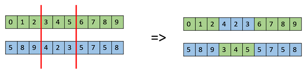
- Uniform crossing: the value that each position of the new individual is obtained from one of the two parents. Usually, the probability of the value coming from each parent is the same, although it could, for example, be conditioned by one’s fitness. Unlike the previous strategies, with this one, each crossing is generates a single offspring.
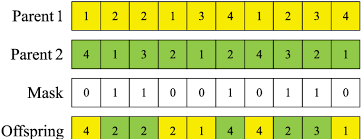
Below, you can see the implementation. The first step consist to extract a copy from one parent to create te new children. Depens of the configuration, the new children receive one porperty from one parent or another.
"""
    This method generates a new individual from two parent individuals using the uniform crossover method.
    """
    def crossover(self, parentA, parentB, crossover_method="uniform"):
        parental_1 = parentA
        parental_2 = parentB
        offspring = copy.deepcopy(parentA)
        offspring.genes = np.repeat(None, self.size)

        if crossover_method == "uniform":
            # Randomly select the positions inherited from parent1 and parent2.
            inheritance_parent_1 = np.random.choice(
                                    a=[True, False],
                                    size=self.size,
                                    p=[0.5, 0.5],
                                    replace=True
                                )
            inheritance_parent_2 = np.logical_not(inheritance_parent_1)

            # Transfer values to the new individual.
            offspring.genes[inheritance_parent_1] = parental_1.genes[inheritance_parent_1]
            offspring.genes[inheritance_parent_2] = parental_2.genes[inheritance_parent_2]

        if crossover_method == "single_point":
            crossover_point = np.random.choice(a=np.arange(1, self.size - 1), size=1)
            crossover_point = crossover_point[0]
            offspring.genes = np.hstack((parental_1.genes[:crossover_point], parental_2.genes[crossover_point:]))

        # The sum of the individual's weights must be 1
        if sum(offspring.genes) != 1:
            offspring.genes = offspring.genes / np.sum(offspring.genes)

        return offspring
Mutation method
Fitting function
To understand optimization algorithms, we first need to understand the concept of minimization. Maximization is a similar concept to optimization - let’s say we have a simple equation y = x2 - the idea is we’re trying to figure out what value of x will maximize y, in this example Infinite. This idea of a maximixer will allow us to build an optimizer.
In our case we’re trying to find a portfolio that maximizes the Sharpe Ratio. To achieve the goal of maximizes the Sharpe Ratio function we must create some functions that will generate the expected portfolio performance, performance weights, and the standard deviation of the portfolio, sharpe ratio and many random portfolios.
First, In order to simulate thousands of possible allocations for our simulation we’ll be using a few statistics, one of which is mean daily return. For this we’re going to switch to using logarithmic returns instead of arithmetic returns. In the world of finance, the arithmetic mean is not usually an appropriate method for calculating an average.
Then, into __shrape function we calculate return, volatility, and the Sharpe Ratio as of the logarithmic mean. Also, the method has one param, that are the weight of every component of the portfolio generated on the current iteration
Fitness method
    def __sharpe(self, genes):
        # calculate annualized portfolio return
        exp_ret = np.sum((self.df.mean() * genes) * 252)
        # calculate annualized portfolio volatility
        exp_vol = np.sqrt(np.dot(genes.T, np.dot(self.df.cov() * 252, genes)))
        sharpe = exp_ret / exp_vol

        return {'exp_ret': exp_ret, 'exp_vol': exp_vol, 'sharpe': sharpe}

    def __fitness(self, genes):
        return self.__sharpe(genes)

    def calculateFitness(self):
        # Determine the fitness of an individual. Higher is better.

        self.biggest = 0
        self.second = 0
        self.avg_fitness = 0

        for ix in range(len(self.pop)):
            # Fitness score is the Sharpe ratio
            fitness = self.__fitness(self.pop[ix].genes)

            self.pop[ix].fitness = fitness['sharpe']
            self.pop[ix].exp_vol = fitness['exp_vol']
            self.pop[ix].exp_ret = fitness['exp_ret']

            self.avg_fitness += float(self.pop[ix].fitness) / len(self.assets)
            # Save the 2 highest fitness for reproduction
            if self.pop[ix].fitness > self.pop[self.biggest].fitness:
                self.biggest = ix
            elif self.pop[ix].fitness > self.pop[self.second].fitness:
                self.second = ix

        # Calculate average fitness
        self.avg_fitness = (self.avg_fitness / len(self.pop)) * 100.0
Early stop
When you are solving a problems without know te results, one of the problems are that you are not know when te algorithm has finished. For this, I have develop a param into main function to detect if during the last ‘stop_rounds’ generations the difference absolute among better individuals is not higher than the value of ‘stop_tolerance’, the algorithm is stopped. The ‘stop_rounds’ is the number of consecutive generations with no minimum improvement to activate the early stop. And the ‘stop_tolerance’ is the minimum value that must have the difference of consecutive generations to consider that there is change
    def optimization(self, mutation_rate=0.1, n_generations=10, early_stopping=False, stopping_rounds=0, stopping_tolerance=0.01, crossover_method="uniform"):
        """
        This method performs the optimization process of a population.
        Parameters

        mutation_rate : `float`, optional
            probability that each position of the individual will mutate.
            (default 0.1)

        n_generations : `int`
            number of repetitions for validation. The method used is
            `ShuffleSplit` from scikit-learn. (default 10)

        early_stopping : `bool`, optional
            if during the last `stopping_rounds` generations the absolute
            difference between the best individuals is not greater than
            the value of `stopping_tolerance`, the algorithm stops and no
            new generations are created. (default ``False``)

        stopping_rounds : `int`, optional
            number of consecutive generations without minimum improvement
            to trigger early stopping. (default ``None``)

        stopping_tolerance : `float` or `int`, optional
            minimum value that the difference of generation

        crossover_method : {"uniform", "single_point"}
            crossover method used.
        """
        generation = 0
        start = time.time()

        # EVALUATE INDIVIDUALS OF THE POPULATION
        # ------------------------------------------------------------------
        while generation in np.arange(n_generations):
            print("-------------")
            print("Generation: " + str(generation))
            print("-------------")
            self.calculateFitness()

            # STORE GENERATION INFORMATION IN HISTORY
            # ------------------------------------------------------------------
            self.historic_best_fitness.append(copy.deepcopy(self.pop[self.biggest].fitness))
            self.historic_best_predictor.append(copy.deepcopy(self.pop[self.biggest].genes))
            self.historic_best_return.append(copy.deepcopy(self.pop[self.biggest].exp_ret))
            self.historic_best_stdev.append(copy.deepcopy(self.pop[self.biggest].exp_vol))

            # CALCULATE ABSOLUTE DIFFERENCE WITH RESPECT TO THE PREVIOUS GENERATION
            # ------------------------------------------------------------------
            # The difference can only be calculated from the second
            # generation.
            if generation == 0:
                self.abs_difference.append(None)
            else:
                difference = abs(self.historic_best_fitness[generation] - self.historic_best_fitness[generation-1])
                self.abs_difference.append(difference)

            # STOPPING CRITERION
            # ------------------------------------------------------------------
            # If during the last n generations, the absolute difference between
            # the best individuals is not greater than the value of stopping_tolerance,
            # the algorithm stops and no new generations are created.
            if early_stopping and generation > stopping_rounds:
                last_n = np.array(self.abs_difference[-(stopping_rounds):])
                if all(last_n < stopping_tolerance):
                    print("Algorithm stopped at generation "
                        + str(generation)
                        + " due to lack of minimum absolute change of "
                        + str(stopping_tolerance)
                        + " during "
                        + str(stopping_rounds)
                        + " consecutive generations.")
                    break

            self.nextGeneration()
            generation += 1

        optimal_value_index = np.argmax(np.array(self.historic_best_fitness))
        optimal_predictors = self.historic_best_predictor[optimal_value_index]
        optimal_fitness_value = self.historic_best_fitness[optimal_value_index]
        optimal_returns = self.historic_best_return[optimal_value_index]
        optimal_volatility = self.historic_best_stdev[optimal_value_index]

        results_df = pd.DataFrame({
            "historic_best_fitness": self.historic_best_fitness,
            "historic_best_predictor": self.historic_best_predictor,
            "historic_best_return": self.historic_best_return,
            "historic_best_stdev": self.historic_best_stdev
        })

        end = time.time()
        print("-------------------------------------------")
        print("Optimization completed " + datetime.now().strftime('%Y-%m-%d %H:%M:%S'))
        print("-------------------------------------------")
        print("
Early stop method
Case studies
As output of the genetic algorithm can be visualized for each generation, which has been the best combination along with the list of the best weights. We select an investment portfolio formed by Cellnex Telecom, S.A.(MTS.MC) , ArcelorMittal (MTS.MC), Ferrovial, S.A. (FER.MC) and Banco Santander, S.A. (SAN.MC).
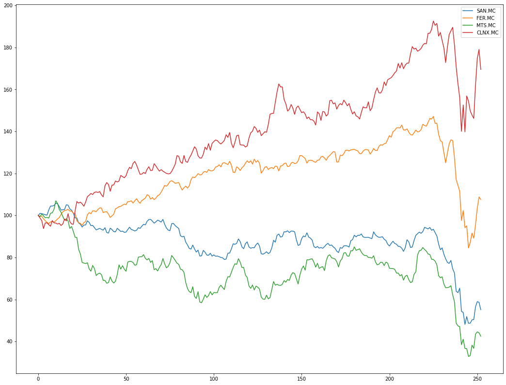
Daily prices of the companies for 1 year
If we select an investment portfolio formed by Cellnex Telecom, S.A.(MTS.MC) , ArcelorMittal (MTS.MC), Ferrovial, S.A. (FER.MC) and Banco Santander, S.A. (SAN.MC). The results are as follows: 0% Telecom and 0,1% ArcelorMittal, 0% Ferrovial and 99% Banco Santander . If we look at the allocations, it makes perfect sense since the strongest company is Santander and it has a much higher return than the rest and therefore should be given more weight to investment. On the other hand, the companies with a negative average are assigned less than 1% of the total weightof the portfolio.
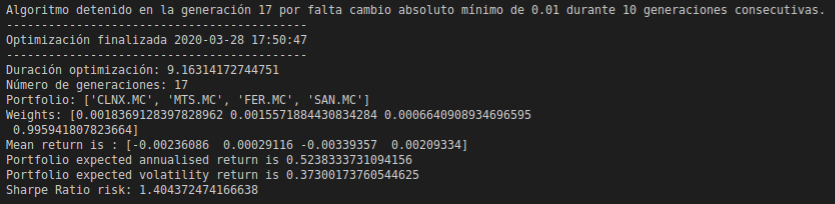
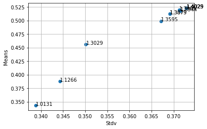
Output generate for the softwareRatio value for every portofolio
Bibliography
- Rodríguez, M. P., Cortez, K. A., Méndez, A. B. y Garza, H. H. (2015). Análisis de portafolios por sectores mediante el uso de algoritmos genéticos: caso aplicado a la Bolsa Mexicana de Valores. Contaduría y Administración, 60(1), 87-112.
- Castro Enciso S. Fernando, “Creación de Portafolios de Inversión utilizando Algoritmos Evolutivos Multiobjetivo”, Tesis de Licenciatura, Centro de Investigación y Estudios Avanzados del Instituto Politécnico Nacional, México, D.F, (2005).